Examining the logs
When dolphot has finished running, we first verify the success of the run by examining several of the diagnostic files produced during the reduction, as well as inspection of the output photometric catalog.
The first file we may want to examine is the log file where we captured dolphot’s standard output. This log contains useful information about much of the reduction. The first step is to make sure the images were read in correctly and the CCD parameters were set to reasonable values. In the case of our M92 example, our log reports:
Reading IMAGE extension: 2048x2048
  GAIN=2.08 EXP=268s NOISE=11.43 BAD=-628.85 SAT=293158.00
Reading IMAGE extension: 2048x2048
  GAIN=2.02 EXP=268s NOISE=10.52 BAD=-284.37 SAT=366377.97
Reading IMAGE extension: 2048x2048
  GAIN=2.17 EXP=268s NOISE=10.34 BAD=-508.59 SAT=276958.84
Reading IMAGE extension: 2048x2048
  GAIN=2.02 EXP=268s NOISE=10.60 BAD=-162.74 SAT=276123.22
Reading IMAGE extension: 2048x2048
  GAIN=2.01 EXP=268s NOISE=11.77 BAD=-1178.38 SAT=279833.47
Reading IMAGE extension: 2048x2048
  GAIN=2.14 EXP=268s NOISE=12.77 BAD=-390.42 SAT=333020.91
Reading IMAGE extension: 2048x2048
  GAIN=1.94 EXP=268s NOISE=11.85 BAD=-215.73 SAT=341808.75
...
If anything did not proceed correctly with the pre-processing routines (e.g., nircammask) it will usually be evident in the image parameters. Make sure that GAIN, BAD and SAT are reasonable values (i.e., close to unity, moderately negative numbers, and large positive numbers, respectively).
After the images are read in correctly, a common source of poor photometry is the astrometric alignment of the frames. DOLPHOT calculates geometric transformations between each of the science frames and the reference image. If the transformations are not sufficiently accurate, the photometry will typically be suboptimal. In our M92 example, we can check the aligment in the log file:
72112 stars for alignment
image 1: 4073 matched, 3953 used, 0.08 0.03 1.000000 0.00000 -0.003, sig=0.08
image 2: 4090 matched, 3999 used, 0.11 -0.06 1.000000 0.00000 0.004, sig=0.10
image 3: 11001 matched, 10506 used, 0.02 0.05 1.000000 0.00000 0.001, sig=0.11
image 4: 11557 matched, 10969 used, 0.04 -0.05 1.000000 0.00000 -0.003, sig=0.11
image 5: 4759 matched, 4677 used, 0.06 0.04 1.000000 0.00000 -0.003, sig=0.12
image 6: 4973 matched, 4861 used, 0.09 -0.02 1.000000 0.00000 0.003, sig=0.10

...
The two key metrics to monitor here are the number of matched stars for each image, and the sig values, which is the rms residual in px around the best-fit transformation. The acceptable values for matched stars and sig depend somewhat on how dense the stellar field is and what camera is being analyzed. For a moderately populated NIRCam field, we want most of the images to have at least 100 matched stars and sig values below 0.30.
Tip
If the alignment solutions are sub-optimal, you may first try to increase the AlignTol parameter. Alternatively, you may try a different reference image.
Once we have made sure that the frames are properly aligned, we may wish to assess that the subsequent steps of the reduction have been successful. This includes making sure that enough PSF stars have been identified:
4648 PSF stars; 735524 neighbors
Central pixel PSF adjustments:
 image 1: 295 stars, -0.004390
 image 2: 272 stars, -0.002881
 image 3: 258 stars, -0.017773
 image 4: 267 stars, -0.006303
 image 5: 268 stars, -0.021525
 image 6: 206 stars, -0.024222
...
In a moderately populated NIRCam field, having at least 100 PSF stars per image would be desirable. Besides the number of PSF stars used for every image, dolphot also lists the average PSF adjustment. This is the fractional flux difference in the central PSF pixel, between the model PSFs and the profile of the PSF stars. Ideally, this number should be as close to 0 as possible. Absolute PSF adjustments below 0.05 should provide enough photometric accuracy for most applications.
Finally, the log file contains details about the aperture correction step. Again, make sure that at least 100 stars are used in each image:
Aperture corrections:
image 1: 200 total aperture stars
  200 stars used, -0.001 (-0.001 +/- 0.000, 0.001)
  199 stars used, -0.005 (-0.006 +/- 0.000, 0.001)
  200 stars used,  0.120 (0.119 +/- 0.000, 0.001)
image 2: 200 total aperture stars
  200 stars used, -0.001 (-0.002 +/- 0.000, 0.001)
  198 stars used, -0.004 (-0.005 +/- 0.000, 0.001)
  200 stars used,  0.122 (0.122 +/- 0.000, 0.001)
image 3: 200 total aperture stars
  200 stars used, -0.003 (-0.003 +/- 0.000, 0.001)
  198 stars used, -0.008 (-0.009 +/- 0.000, 0.001)
  200 stars used,  0.121 (0.120 +/- 0.000, 0.001)
image 4: 200 total aperture stars
  200 stars used, -0.001 (-0.001 +/- 0.000, 0.001)
  198 stars used, -0.003 (-0.003 +/- 0.000, 0.001)
  200 stars used,  0.117 (0.117 +/- 0.000, 0.001)
image 5: 200 total aperture stars
  200 stars used, -0.005 (-0.006 +/- 0.000, 0.001)
  197 stars used, -0.009 (-0.010 +/- 0.000, 0.001)
  200 stars used,  0.124 (0.124 +/- 0.000, 0.001)
image 6: 200 total aperture stars
  200 stars used, -0.005 (-0.005 +/- 0.000, 0.001)
  199 stars used, -0.011 (-0.011 +/- 0.000, 0.001)
  200 stars used,  0.118 (0.118 +/- 0.000, 0.001)
...
If inspection of the log file does not reveal any anomaly, the reduction has most likely been successful. When dolphot is run with the following syntax:
> dolphot <outputname> <options> > <logfile>
Additional diagnostic files are generated, using outputname as root.
The outputname.warnings contains potential anomalies that have been encountered during reduction and could have compromised photometric quality. Be sure to check this file. In our M92 example, M92_example.phot.warnings is empty.
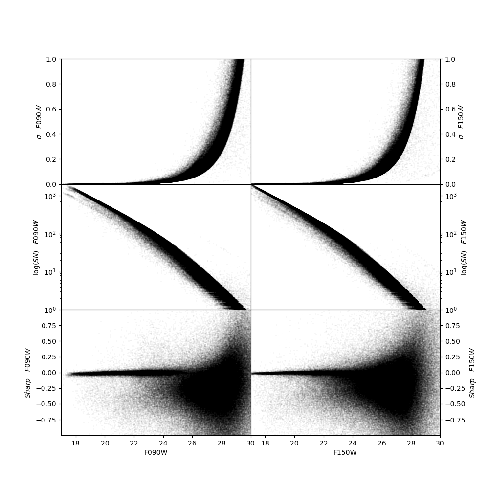
Examining the catalog
The output photometric catalog is stored in the outputname file. This file contains a output line for each point-source identified during the reduction run. For each line, the outputname file contains a long list of outputs. These include photometric measurements and quality flags on each indivual frame, as well as combined photometry from multiple images that use the same filter. The detailed list of all output columns can be found in the outputname.columns file. In our example, these are the first 70 columns of our output file:
1. Extension (zero for base image)
2. Chip (for three-dimensional FITS image)
3. Object X position on reference image (or first image, if no reference)
4. Object Y position on reference image (or first image, if no reference)
5. Chi for fit
6. Signal-to-noise
7. Object sharpness
8. Object roundness
9. Direction of major axis (if not round)
10. Crowding
11. Object type (1=bright star, 2=faint, 3=elongated, 4=hot pixel, 5=extended)
12. Total counts, NIRCAM_F090W
13. Total sky level, NIRCAM_F090W
14. Normalized count rate, NIRCAM_F090W
15. Normalized count rate uncertainty, NIRCAM_F090W
16. Instrumental VEGAMAG magnitude, NIRCAM_F090W
17. Transformed UBVRI magnitude, NIRCAM_F090W
18. Magnitude uncertainty, NIRCAM_F090W
19. Chi, NIRCAM_F090W
20. Signal-to-noise, NIRCAM_F090W
21. Sharpness, NIRCAM_F090W
22. Roundness, NIRCAM_F090W
23. Crowding, NIRCAM_F090W
24. Photometry quality flag, NIRCAM_F090W
25. Total counts, NIRCAM_F150W
26. Total sky level, NIRCAM_F150W
27. Normalized count rate, NIRCAM_F150W
28. Normalized count rate uncertainty, NIRCAM_F150W
29. Instrumental VEGAMAG magnitude, NIRCAM_F150W
30. Transformed UBVRI magnitude, NIRCAM_F150W
31. Magnitude uncertainty, NIRCAM_F150W
32. Chi, NIRCAM_F150W
33. Signal-to-noise, NIRCAM_F150W
34. Sharpness, NIRCAM_F150W
35. Roundness, NIRCAM_F150W
36. Crowding, NIRCAM_F150W
37. Photometry quality flag, NIRCAM_F150W
38. Total counts, NIRCAM_F277W
39. Total sky level, NIRCAM_F277W
40. Normalized count rate, NIRCAM_F277W
41. Normalized count rate uncertainty, NIRCAM_F277W
42. Instrumental VEGAMAG magnitude, NIRCAM_F277W
43. Transformed UBVRI magnitude, NIRCAM_F277W
44. Magnitude uncertainty, NIRCAM_F277W
45. Chi, NIRCAM_F277W
46. Signal-to-noise, NIRCAM_F277W
47. Sharpness, NIRCAM_F277W
48. Roundness, NIRCAM_F277W
49. Crowding, NIRCAM_F277W
50. Photometry quality flag, NIRCAM_F277W
51. Total counts, NIRCAM_F444W
52. Total sky level, NIRCAM_F444W
53. Normalized count rate, NIRCAM_F444W
54. Normalized count rate uncertainty, NIRCAM_F444W
55. Instrumental VEGAMAG magnitude, NIRCAM_F444W
56. Transformed UBVRI magnitude, NIRCAM_F444W
57. Magnitude uncertainty, NIRCAM_F444W
58. Chi, NIRCAM_F444W
59. Signal-to-noise, NIRCAM_F444W
60. Sharpness, NIRCAM_F444W
61. Roundness, NIRCAM_F444W
62. Crowding, NIRCAM_F444W
63. Photometry quality flag, NIRCAM_F444W
64. Measured counts, jw01334001001_02101_00001_nrca1_cal (NIRCAM_F090W, 268.4 sec)
65. Measured sky level, jw01334001001_02101_00001_nrca1_cal (NIRCAM_F090W, 268.4 sec)
66. Normalized count rate, jw01334001001_02101_00001_nrca1_cal (NIRCAM_F090W, 268.4 sec)
67. Normalized count rate uncertainty, jw01334001001_02101_00001_nrca1_cal (NIRCAM_F090W, 268.4 sec)
68. Instrumental VEGAMAG magnitude, jw01334001001_02101_00001_nrca1_cal (NIRCAM_F090W, 268.4 sec)
69. Transformed UBVRI magnitude, jw01334001001_02101_00001_nrca1_cal (NIRCAM_F090W, 268.4 sec)
70. Magnitude uncertainty, jw01334001001_02101_00001_nrca1_cal (NIRCAM_F090W, 268.4 sec)
...
While the frame-by-frame photometric output (columns 64 and below, in our example) can be useful for, e.g. variable star work, for the purpose of generating a photometric catlog, we are only interested in the global properties of the source (columns 3-11) and in the combined photometry properties (columns 12-63). For example, we can use these quantities to perform a first inspection of the photometry. In our example, we can see in the plot below that the photometric error and the signal-to-noise follow expected and well-defined trends as function of source magnitude. The sharpness values (see Culling the catalog for more details) are also close to 0 for a large range of magnitudes, demonstrating the good outcome of the PSF-photometry.